Analysing the sentiment behind tweets is a technical challenge: They are often sarcastic, full of abbreviations and poor spelling, and even contain made-up words. I recently learned how to do sentiment analysis with Python, Elasticsearch and Kibana. To test my new skills, I analysed tweets about Donald Trump. Here's how I went about this.
I wanted to do a sentiment analysis of tweets to get a "feel" for the tools being used in my new team. In sentiment analysis, you:
- Tokenise text: This means splitting the text into words
- Remove stopwords
- Do Part-of-speech (POS) tagging: This allows you to select only significant features in the text
- Pass the features to a sentiment classifier which then determines the sentiment of the text
All of this aims to get a general sense of whether people have a positive or negative attitude about a specific topic.
To get a better understanding of sentiment analysis, I needed a large volume of tweets with different sentiments. In other words, I needed tweets on a divisive, polarising topic. And what current topic is more divisive and polarising than Donald Trump?
The goal of my analysis was to see which US states were feeling positive or negative about Trump.
I knew this would be an interesting problem to solve:
- Tweets are short (limited to 140 characters): Therefore, users need to stay focused on the message they wish to convey. In theory, this makes it easier to analyse tweets than larger text such as blogs or newspaper articles. It's also relatively easy to get a large number of different texts from Twitter.
- There are fewer tokens to analyse: At the same time, if tokens in the very short tweet vary wildly in sentiment, the nett result could be skewed.
- Tweets often contain slang or abbreviations: Words that are not in an official corpus make it difficult to determine if the words are positive or negative.
- Sarcasm is prevalent in tweets: It is very difficult to detect sarcasm with sentiment analysis. The text often needs to be reviewed by a person to determine if it is sarcastic. Although a lot of research has been done to automatically identify sarcasm, many researchers do not think sarcasm can be detected reliably yet.
- There are ambiguous negative words: "That backflip was so sick" is really a positive statement so the context of words like "sick" needs to be thoroughly understood and tagged accordingly.
Before I could dive into the actual sentiment analysis of tweets about Trump, I first needed to collect the tweets and prepare them for analysis, and find and set up a tool to visualise the results. Visualisations would make it a lot easier for me to draw meaningful conclusions from the results. With everything in place, I would be able to create the actual code to do sentiment analysis.
I created a Python project to collect tweets, add tweets to an ElasticSearch index, and perform sentiment analysis on the tweets using the TextBlob library. I used Kibana to create a dashboard to visualise the results of the analysis.
Here's how I went about each step, but if you want to skip to the TL;DR version and see the end product, check out the GitHub repo for my project.
Step 1: Getting access to the tweets using the Twitter API
Twitter makes it easy for developers to interact with tweets and user data. In order to use them in an application, you need to apply for a developer account and create an app on the Twitter developer portal. After this is completed, you can generate consumer keys and access tokens that are required to authenticate your application.
In order to access tweets using Python, I used Tweepy. Tweepy is a Python library that allows you to interact with tweets. It makes it easier to use the Twitter streaming API because it handles the authentication, connection, creation and destruction of a session, reads incoming messages, and partially routes messages.
Creating a Twitter stream filter
When creating a Twitter stream it is possible to add a filter. You can specify which terms it needs to search for: Any tweets that don't contain the specified words, hashtags or at-tags are ignored.
To determine which tweets were about Donald Trump, I created a filter with the following search terms:
- @realDonaldTrump - People tag Donald Trump in tweets regularly.
- #donaldtrump - This is the hashtag commonly used when tweeting about Donald Trump.
- #trump - Another hashtag used regularly.
- #potus - This is the hashtag used for the president of the United States of America.
I ran this project during the month of November 2018 and the tweets were collected in real-time. Each tweet document was saved as is, including all the metadata, as a JSON document.
Step 2: Filtering indexed tweets by tweet location
Because I wanted to analyse the sentiment of tweets by US state, I needed to find the location of tweets. The problem with choosing a divisive topic such as Donald Trump is that everyone with a Twitter account across the globe has an opinion about him. This meant that I needed to filter only the tweets from within the United States.
Each tweet has numerous fields, some of which can be used to determine its location. One of these fields is 'place' which indicates that the tweet is associated with but not necessarily originating from a place.
Each tweet also contains a user object with different fields such as user-defined location for the specific account. This again is not necessarily a location, nor is it machine-parseable. Because it is controlled by the user, I needed to process the data to determine in which state the user resides.
That's how it looked in the actual code:
def find_place(self, tweet):
        """Find the location of the tweet using 'place' or 'user location' in tweets
        :param tweet: JSON tweet data to process
        :return: 2 letter state abbreviation for tweet location"""

        # Find location from place
        if tweet['place'] is not None:
            state = tweet['place']['full_name'].split(',')[1].strip()
            return state
        # Find location from user location
        elif tweet['user']['location'] is not None:
            # Split location into single word tokens
            places_splits = tweet['user']['location'].replace(',', ' ').split(' ')
            for place in places_splits:
                # Remove leading and trailing whitespaces
                place = place.strip()
                # Determine if the state abbreviation or full state name is in location
                for key, value in states.items():
                    if key.lower() == place.lower():
                        return key
                    if value.lower() == place.lower():
                        return key
            return None
        else:
            return None
Step 3: Making the tweets indexable using Elasticsearch
Elasticsearch is fast and makes working with text data very convenient. I created a Twitter stream listener class to get tweets using the Twitter API. I then converted each tweet to a JSON object in Python using the json.loads() function and added it to the Elasticsearch index.
def on_data(self, data):
        """
        Process tweet data from the twitter stream as it is available.
        :param data: Tweet data from twitter stream
        :return: boolean - false if something broke such as the stream connection, else true
        """
        # Clean up tweet
        try:
            tweet = json.loads(data)
        except:
            self.logger.error("Unable to parse tweet to json")

        try:
            # Add tweet json to Elasticsearch
            self.es.index(index='twitter_data', doc_type='twitter', body=tweet, ignore=400)
        except:
            self.logger.error("Unable to add tweet to Elasticsearch")
            return False
Step 4: Performing sentiment analysis
The sentiment analysis only starts after all the indexing is done. That's why it makes sense to schedule it at times when fewer tweets are generated, such as at night.
To perform the sentiment analysis, I used the TextBlob Python library which can be used to process text. It provides a simple API for diving into common natural language processing (NLP) tasks such as part-of-speech tagging, noun phrase extraction, sentiment analysis, classification and translation.
It contains two types of analysers:
PatternAnalyzer
The default analyser is the PatternAnalyzer. It uses the same implementation as the pattern library and returns results as a named tuple of the form:
Sentiment(polarity, subjectivity, [assessments])
where [assessments] is a list of the assessed tokens and their polarity and subjectivity scores.
def analyse_sentiment_textblob(self, tweet):
        """Determine sentiment using TextBlob PatterAnalyzer
        :param tweet: tweet text as string
        :return: Tweet sentiment value (determined from PatternAnalyzer polarity)"""
        analysis = TextBlob(tweet)
        if analysis.sentiment.polarity > 0:
            return 1
        elif analysis.sentiment.polarity == 0:
            return 0
        else:
            return -1
NaiveBayesAnalyzer
The other analyser is a NaiveBayesAnalyzer. This analyser is trained on a movie review dataset. It also returns results as a named tuple of the form:
Sentiment(classification, p_pos, p_neg)
where classification is the positive or negative, p_pos is the probaibilty that the text is positive, an p_neg is the probability thet the text is negative.
def analyse_sentiment_textblob_nb(self, tweet):
        """Determine sentiment using TextBlob NaiveBayesAnalyzer
        :param tweet: tweet text as string
        :return: tweet sentiment value (determined from NaiveBayes classification)"""
        analysis = TextBlob(tweet, analyzer=NaiveBayesAnalyzer())
        if analysis.sentiment.classification == 'pos':
            return 1
        else:
            return -1
For my Twitter analysis, I decided to compare both methods so that I could better understand the differences.
Step 5: Looking at the analysis results
Visualising the results with Kibana
Kibana is an open source analytics and visualisation platform designed to work with Elasticsearch. Its primary goal is to make it easy to understand large volumes of data. Kibana allows you to:
- Visualise geospatial data on a map
- Perform advanced time series analysis on data
- Analyse relationships in data using graph exploration
- Explore anomalies using unsupervised machine learning features
- Create dashboards
- View your data in real time
Being able to view data in real time is handy for tweet sentiment analyses, because it allows you to get a feel for how the sentiment of states changes over time. This can happen quite quickly depending on real-world factors such as news broadcasts and other world events, which, by the way, is also generally applicable to other sentiment analysis projects such as determining the sentiment of users of a software platform or online shoppers.
Who tweeted about Trump the most?
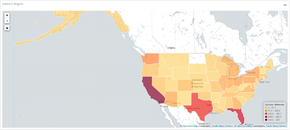
The above graphic shows the region map I created to show how many tweets were from which states. As you can see, most of the tweets came from California, Florida and Texas.
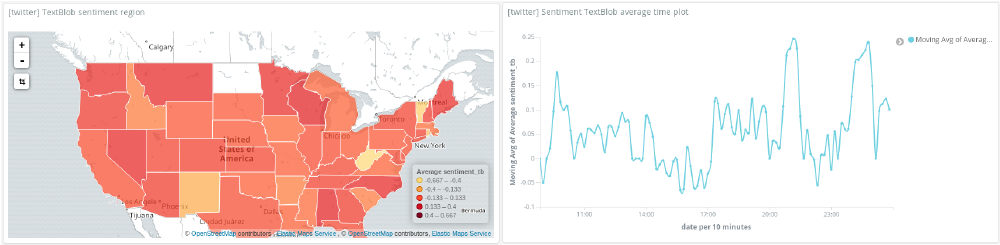
Who is most positive and negative about Trump — and how has sentiment towards him changed over time?
The visualisations below show the results of the Textblob PatternAnalyzer. On the left, you can see the sentiment for each state. The darker red the state, the more negative the tweets. On the right you can see the moving average of the overall sentiment of tweets. From the region map we can see that New Mexico is the most positive about Trump with an average sentiment between 0.4 and 0.667. The majority of states where more neutral to negative with average sentiments below 0.133.
The NaiveBayes analyser, however, shows quite different results: New Mexico is again a positive state, along with West Virginia and Maine with average sentiments each between 0.16 and 0.45. The most negative states are Colorado, Kansas and South Dakota. The majority of states were more neutral to negative with average sentiments below -0.127
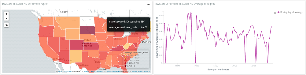
Looking at the amount of movement in the average sentiment over time shows how quickly the sentiment on a topic can change. It is interesting to note that the project was run during the American Midterm elections in November 2018. This accounts for large swings in the average sentiment.
Eagle-eyed readers will also note that the colours on the region maps do not match the results I just mentioned. Kibana has predefined colour ranges to use with region maps. In order to match darker red to more negative tweets (red = bad), I had to invert the average sentiment for the graph.
Comparing NaiveBayes and Pattern Analyser
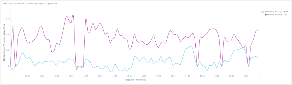
Now, looking at these results, which analyser is better? Comparing the two methods' overall average sentiment results, it becomes clear that the NaiveBayes analyser (purple) marks more tweets as positive than the Pattern Analyser (blue).
To determine which analyser performed better, I selected a sample of 50 tweets. I analysed each of the tweets myself to determine the sentiment. Then I compared the results of the two analysers to the sentiment I decided on.
Looking at individual tweet results was very entertaining. Each of the analyses struggled with the same problems, but for different tweets:
- "Donald you have the brain of a six year old"
- Marked as positive by NaiveBayesAnalyzer
- "I see they've given you the phone back"
- Marked as neutral by PatternAnalyzer
- "The GOP=Gutless Obtuse Pathetic"
- Marked as positive by NaiveBayesAnalyzer
PatternAnalyzer accuracy
Double-checking the PatternAnalyser, I found that it was correct about 34% of the time, incorrect about 23% of the time, and marked about 43% of the tweets as neutral.
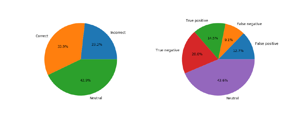
Looking at the results more closely, I realised that it had incorrectly marked about 9% of tweets as negative and about 13% as positive. This shows that the analysis is not overly biased to marking tweets as positive or negative.
The NaiveBayes accuracy
Taking a look at the Naive Bayes based analysis of the same set of tweets, I found that about 53% of the tweets were correctly marked.
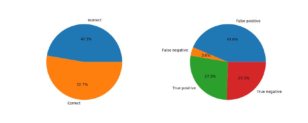
Upon closer inspection, the Naive Bayes based analysis incorrectly marked 3% of tweets as negative and more than 46% incorrectly as positive. This shows that the Naive Bayes analysis is heavily biased towards marking tweets as positive when they are not.
All in all, I realised that both methods seem to have the same difficulties when analysing tweet sentiments:
- Abbreviations
- Tweets that appear both positive and negative at the same time
- Sarcasm
- New words
- Spelling
- Classifying a lot of tweets as neutral
- Context
- Profanity
- Very short tweets (1-2 words)
I also realised that I still have a lot to learn. In order to increase the accuracy of the analysers, I would need to create a proper text classification system to do things like tokenisation, parts-of-speech tagging and train models. However, this was a great way to get started with sentiment analysis and text processing.
Anri is a software engineer with a passion for machine learning, artificial intelligence and competitive programming. She loves learning new techniques and methods and applying them to quirky and fun problems.